Page 81 - Azerbaijan State University of Economics

J-CURVE AND THE MARSHALL-LERNER CONDITION - THE CASE OF AZERBAIJAN

integration forms for the export and for the import equations. For this

paper, the following VECM specification is used:
∆Z t=μ t + ∑ jγ j∆Z t-j + ∏X t-1 + u t (4)

where, Zt is a vector of endogenous variables, μ t – deterministic

component, γ j – matrix of coefficients, ∏=αβ’, where α is the parameter

of speed adjustment, and β’ is the vector of co integration, u t – matrix of
residuals.

Finally, IRFs of the exports and imports will demonstrate the
short-run dynamics of the two aggregates, while an IRF on the trade

balance (X-IM) will capture the J-curve phenomenon.

4. Empirical Results

Unit Root Tests
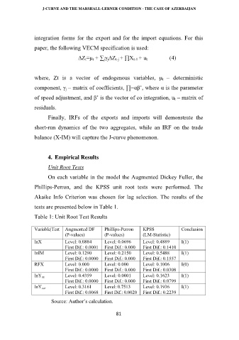
On each variable in the model the Augmented Dickey Fuller, the

Phillips-Perron, and the KPSS unit root tests were performed. The
Akaike Info Criterion was chosen for lag selection. The results of the

tests are presented below in Table 1.

Table 1: Unit Root Test Results

Variable|Test Augmented DF Phillips-Perron KPSS Conclusion
(P-values) (P-values) (LM-Statistic)
lnX Level: 0.0884 Level: 0.0696 Level: 0.4889 I(1)
First Dif.: 0.0001 First Dif.: 0.000 First Dif.: 0.1410
lnIM Level: 0.1290 Level: 0.2150 Level: 0.5488 I(1)
First Dif.: 0.0000 First Dif.: 0.000 First Dif.: 0.1557
RFX Level: 0.000 Level: 0.000 Level: 0.1006 I(0)
First Dif.: 0.0000 First Dif.: 0.000 First Dif.: 0.0308
Level: 0.4359 Level: 0.0001 Level: 0.1623 I(1)
lnY az
First Dif.: 0.0000 First Dif.: 0.000 First Dif.: 0.0799
Level: 0.3161 Level: 0.7513 Level: 0.1936 I(1)
lnY eur
First Dif.: 0.0068 First Dif.: 0.0020 First Dif.: 0.2239
Source: Author’s calculation.

81