Page 19 - Azerbaijan State University of Economics

N.Akimov., S.Baizakov., A. Oinarov., E.Utembayev: The analysis of the macroeconomic
dynamics and assessment of smart factors’ inputs to the balanced growth rates

The solution for this problem, according to A. Granberg, has been seen in the
close interconnection in the assessment of the ratios between the two subsets.
For the purposes of the study of such interconnectedness, he has carried out
the analyses of the three types of economic development that differ in their pre-set
rt
growth rates of consumption r on the trajectory с(t) = с(0)e , and in the dynamics
of the rates of production consumption . For a start, it has been assumed that
the parameters of the macro - technology are: coefficients А and В, and they remain
unchanged, in time.
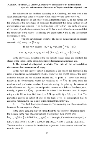
1. The first development scenario. The rate of the accumulation remains
constant:

In this case, because

then and

In the above case, the rates of the two subsets remain equal and constant; the
shares of the subsets in the gross domestic product remain unchanged, also.
2. The second development scenario. The rate of the accumulation
decreases as the consequence of r> .
In this case, the share of subset II increases at the cost of the decrease in the
rates of production accumulations: > . However, the growth rates of the gross

domestic product and the national income fall. At point t 1 these rates nullify.
Earlier in the development: under the condition of t = <t 1 the rates reach the

maximum and production in subset I starts decreasing. At point t 2 the volume of
national income and of gross national product become zero. Prior to the above point,
namely, at point t = <t 2 — production in subset I also becomes zero. Example:

using r = 0, 08 we then find that = 3,24, t 1= 4,98, = 9,8, t 2 = 11,16. The
prevailing growth in subset II due to the high levels of consumption has its
economic rationale, but that is only at insignificant time intervals.
3. The third development scenario. The increasing rate of accumulations
is seen as the consequence of r< .
In the above case, the share of subset I and the rate in subset I increase due to
the increase in the rates of accumulations. The limits of their growth are :
Example, if r = 0,04 we have p 1(5) =

0,11, p 1 (10) = 0,185, p 1 (20) = 0,275, (5) = 0,73, (10) = 0,82, (20) = 0,97.

The feature that is common for the obtained trajectories is the constant nature of the
rates in subset II.

19