Page 61 - Azerbaijan State University of Economics

THE JOURNAL OF ECONOMIC SCIENCES: THEORY AND PRACTICE, V.70, # 2, 2013, pp. 32-66

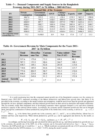
Table -7- : Demand Components and Supply Sources in the Bangladesh
Economy during 2011-2017, in Tk billion ( 2005-06 Price)

Demand Side of the Economy Supply Side
Private Government Changes
FY GFCF Exports GDP Imports
Consumption Consumption in Stock
2011 4067.0 555.2 1421.1 -150.4 1239.3 5623.2 1509.0
2012 5121.7 764.3 1528.7 -1085.8 1541.0 6003.4 1866.5
2013 6048.9 887.7 1684.3 -1873.9 1790.5 6422.4 2115.1
2014 6908.6 1002.7 1803.6 -2526.8 2083.8 6871.1 2400.7
2015 7750.3 1122.4 1999.4 -3199.2 2429.0 7368.4 2733.5
2016 8605.1 1256.6 2123.5 -3812.9 2835.0 7896.6 3110.6
2017 9506.9 1417.5 2371.1 -4569.4 3313.1 8486.5 3552.7
The Compound Annual 15.2 16.98.0 8.9 76.6 17.8 7.1 15.3
1
Growth Rate (%)

Table -8-: Government Revenue by Main Components for the Years 2011-
2017 in Tk billion
Non-
Total Direct/Inc Customs Value-Added
FY Tax
Revenue ome Tax Duty Tax (VAT)
Revenue
2011 537.6 175.0 73.3 199.1 90.2
2012 587.3 153.9 80.6 244.7 108.1
2013 650.3 169.1 82.6 283.0 115.6

2014 710.6 185.8 84.6 316.5 123.7
2015 775.6 204.9 86.7 351.3 132.6
2016 840.5 225.8 88.9 383.6 142.1
2017 914.9 249.8 91.2 421.1 152.8
Annual Growth
Rate (%) 9.2 6.1 3.7 13.2 9.1

1 It is worth mentioning here that the compound annual growth rate of the Bangladesh economy over the coming six
financial years (2012-2017), measured according to the labour productivity and labour-force growth rates, that likely to be
prevailed in the economy, according to the model solution and assumption, would be much lower than the growth rate generated
through the, de facto, demand components, and their deduced growth based on their arrived at elasticities and related coefficients.
This an economic reality that dominated most of developing economies where aggregate demand is over and above domestic
productive capacity of the national labour market. Accordingly, the economy annual compound growth rate that can be brought
s
about, through the combination of labour productivity and growth of the labour force in the economy, is driven as: g e = { L t /
s
L 0 } 1/n -1
s
s
Where; g e is the labour force growth rate in the economy, and L t and L 0 are as defined before, labour force in
terminal and base year respectively. While labour productivity growth (ρ ℓ ), can be aggregated and derived, by the model, as
follows:
t
0
t
0
P ℓ = X t / L t and P ℓ = X 0 /L 0 , and hence; ρ ℓ = { P ℓ / P ℓ } 1/n -1
Accordingly, and having forecasting and calculated the labour growth rate (g e ) and labour productivity growth rate (ρ ℓ )
in the economy, the growth rate of the GDP, (r), of the economy can be forecasted and derived as: ℓog r = ℓog g e * ℓog ρ ℓ
. Therefore, the GDP growth rate (r) would be; r = g e + ρ ℓ Which would give an annual growth rate of (6.1) percent per annum,
as was resulting from the MFFM solution, ( i.e r= 0.023 + 0.039), during the model’s period.

60