Page 35 - Azerbaijan State University of Economics

THE JOURNAL OF ECONOMIC SCIENCES: THEORY AND PRACTICE, V.73, # 2, 2016, pp. 27-41

(a) Coincident regressions where α 1 = β 1 and α 2 = β 2.
(b) Parallel regressions where α 1 ≠ β 1 but α 2 = β 2.
(c) Concurrent regressions where α 1 = β 1 but α 2 ≠ β 2.
(d) Dis-similar regressions where α 1 ≠ β 1 and α 2 ≠ β 2.
However, pooling all the n 1 and n 2 observations together and applying the
dummy variable approach, we estimate a model such as

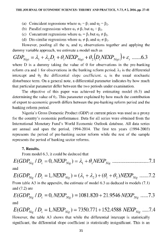
GDP Nigt     D   NEXP Nigt    NEXP Nigt   t ....... 3 . 6
D
1
i
2
1
2
i
where D is a dummy taking the value of 0 for observations in the pre-banking
reform era and 1 for observations in the banking reform period. λ 2 is the differential
intercept and θ 2 the differential slope coefficient. ε t is the usual stochastic
disturbance term. On a general note, a differential parameter indicates by how much
that particular parameter differ between the two periods under examination.
The objective of this paper was achieved by estimating model (6.3) and
determining the value of θ 2. This parameter explained by how much the contribution
of export to economic growth differs between the pre-banking reform period and the
banking reform period.
Nigeria‟s Gross Domestic Product (GDP) at current prices was used as a proxy
for the country‟s economic performance. Data for all series were obtained from the
International Monetary Fund‟s World Economic Outlook database. All data series
are annual and span the period, 1994-2014. The first ten years (1994-2003)
represents the period of pre-banking sector reform while the rest of the sample
represents the period of banking sector reforms.

7. Results.
From model 6.3, it could be deduced that

E (GDP Nig / D  , 0 NEXP Nig )    NEXP Nig .......... .......... ........ 1 . 7
i
1
1
and
E (GDP Nig / D  , 1 NEXP Nig )  (   )  (   )NEXP Nig ....... 2 . 7
2
i
2
1
1
From table A3 in the appendix, the estimate of model 6.3 as deduced in models (7.1)
and (7.2) are
E (GDP Nig / D  , 0 NEXP Nig )  1081 . 820  21 . 9546 NEXP Nig ...... 3 . 7
i
and
E (GDP / D  , 1 NEXP )  7350 . 771 152 . 4588 NEXP ..... 4 . 7
Nig i Nig Nig
However, the table A3 shows that while the differential intercept is statistically
significant, the differential slope coefficient is statistically insignificant. This is an

35