Page 50 - Azerbaijan State University of Economics

THE JOURNAL OF ECONOMIC SCIENCES: THEORY AND PRACTICE, V.82, # 2, 2025, pp. 32-60

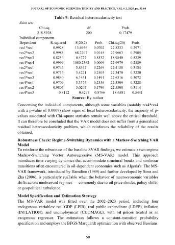
Table 9: Residual heteroscedasticity test
Joint test
Chi-sq df Prob.
218.5928 200 0.17479
Individual components
Dependent R-squared F(20,2) Prob. Chi-sq(20) Prob.
res1*res1 0.9928 13.6956 0.0702 22.8333 0.2971
res2*res2 0.9985 68.2207 0.0145 22.9663 0.2905
res3*res3 0.8254 0.4727 0.8532 18.9840 0.5229
res4*res4 0.9999 1080.2362 0.0009 22.9979 0.2889
res2*res1 0.9746 3.8367 0.2269 22.4158 0.3184
res3*res1 0.9716 3.4221 0.2503 22.3470 0.3220
res3*res2 0.9840 6.1431 0.1491 22.6316 0.3072
res4*res1 0.9709 3.3374 0.2556 22.3309 0.3228
res4*res2 0.9805 5.0207 0.1790 22.5508 0.3114
res4*res3 0.8112 0.4297 0.8766 18.6581 0.5441
Source: By author

Concerning the individual components, although some variables (notably res4*res4
with a p-value of 0.0009) show signs of local heteroscedasticity, the majority of p-
values associated with Chi-square statistics remain well above the critical threshold.
It can therefore be concluded that the VAR model does not suffer from a generalized
residual heteroscedasticity problem, which reinforces the reliability of the results
obtained.

Robustness Check: Regime-Switching Dynamics with a Markov-Switching VAR
Model
To reinforce the robustness of the baseline SVAR findings, we estimate a two-regime
Markov-Switching Vector Autoregressive (MS-VAR) model. This approach
introduces time-varying dynamics that accommodate structural breaks and nonlinear
transitions often encountered in oil-dependent economies such as Algeria's. The MS-
VAR framework, introduced by Hamilton (1989) and further developed by Sims and
Zha (2006), is particularly suiTable when the behavior of macroeconomic variables
shifts across unobserved regimes — commonly due to oil price shocks, policy shifts,
or geopolitical turbulence.

Model Specification and Estimation Strategy
The MS-VAR model was fitted over the 2002–2023 period, including four
endogenous variables: real GDP (LPIB), real public expenditure (LDEP), inflation
(INFLATION), and unemployment (CHOMAGE), with oil prices treated as an
exogenous regressor. The estimation follows a constant-transition probability
specification and employs the BFGS/Marquardt optimization with observed Hessians.

50