Page 24 - Azerbaijan State University of Economics

THE JOURNAL OF ECONOMIC SCIENCES: THEORY AND PRACTICE, V.81, # 2, 2024, pp. 4-29

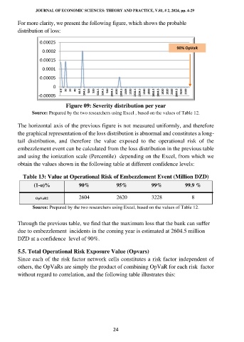
For more clarity, we present the following figure, which shows the probable
distribution of loss:

0.00025
90% OpVaR
0.0002
0.00015
0.0001
0.00005

0
4.5 20 29 40 44.5 504.5 509 520 524.5 524.5 540 1004.5 1020 1304.5 1309 1320 1324.5 1324.5 1340 1800 1804.5 1804.5 1820 1820 2300 2604.5 2620 3100
-0.00005

Figure 09: Severity distribution per year
Source: Prepared by the two researchers using Excel , based on the values of Table 12.

The horizontal axis of the previous figure is not measured uniformly, and therefore
the graphical representation of the loss distribution is abnormal and constitutes a long-
tail distribution, and therefore the value exposed to the operational risk of the
embezzlement event can be calculated from the loss distribution in the previous table
and using the ionization scale (Percentile) depending on the Excel, from which we
obtain the values shown in the following table at different confidence levels:

Table 13: Value at Operational Risk of Embezzlement Event (Million DZD)
(1-α)% 90% 95% 99% 99.9 %

OpVaR2 2604 2620 3228 8
Source: Prepared by the two researchers using Excel, based on the values of Table 12.

Through the previous table, we find that the maximum loss that the bank can suffer
due to embezzlement incidents in the coming year is estimated at 2604.5 million
DZD at a confidence level of 90%.

5.5. Total Operational Risk Exposure Value (Opvars)
Since each of the risk factor network cells constitutes a risk factor independent of
others, the OpVaRs are simply the product of combining OpVaR for each risk factor
without regard to correlation, and the following table illustrates this:

24