Page 37 - Azerbaijan State University of Economics

THE JOURNAL OF ECONOMIC SCIENCES: THEORY AND PRACTICE, V.76, # 2, 2019, pp. 31-45

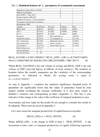
Tab. 1: Statistical features of parametres of econometric assessment

Dependent Variable: REAL_SAVING
Method: Least Squares
Date: 05/02/17 Time: 02:47
Sample (adjusted): 2000 2013
Included observations: 13 after adjustments
Convergence achieved after 18 iterations
MA Backcast: 2000
Variable Coefficient Std. Error t-Statistic Prob.
REAL_GDP 0.205133 0.049011 4.185458 0.0019
AR (1) 0.754837 0.210021 3.594099 0.0049
MA (1) 0.888579 0.158206 5.616610 0.0002
R-squared 0.696393 Mean dependent var 3104.692
Adjusted R-squared 0.635672 S.D. dependent var 787.7870
S.E. of regression 475.5051 Akaike info criterion 15.36581
Sum squared resid 2261051. Schwarz criterion 15.49618
Log-likelihood -96.87774 Hannan-Quinn criteria. 15.33901
Durbin-Watson stat 1.471227
Inverted AR Roots .75
Inverted MA Roots -.89

REAL_SAVING = 0.205133092015 * REAL_GDP + [AR (1) =0.754837146075,
MA(1)= 0.888578691287,BACKCAST=2001,ESTSMPL="2001 2013"] (8)

Where REAL_SAVINGS is the real volume of savings and REAL_GDP is the real
volume of GDP (year-end figures in billions of local currency). The numbers in
brackets below the model's parameters are the t-statistics of the corresponding
parameters. As indicated in Model (8) savings norm is equal to

.

As seen in Appendix 1, t-statistics has statistical significance. Standard errors of
parameters are significantly lower than the values of parameters found by least
squares method (excluding the constant coefficient). It is seen more clearly in
Student’s t-statistics and corresponding p-values (Appendix 1). This fact is also
indicative of the change in the value of the coefficient of marginal propensity to save.

Assessments and tests made for the model (8) are enough to consider this model to
be adequate. These tests are given in appendix 1.

Let’s now assess the marginal productivity of capital based on real data:

∆ _ = ∗ _ (9)

Where ∆ _ is the change in GDP at time t, _ is the
investment at time t and is marginal productivity of capital. Following regression

37